In this project, we added additional features to our ray tracer from Project 3-1. For the project, we used the staff binaries to give ourselves the basic backbone from project 3-1. There were four parts to the project: Mirror and Glass Materials, Microfacet Material, Environment Light, and Depth of Field; however, we only had to do two parts. We chose parts 1 and 4. In part 1, we implemented mirror and glass models with both reflection and refraction. In part 4, we simulated a thin lens to enable the depth of field effect, instead of having everything be in focus like in previous projects.
Part 1: Ray Generation and Intersection
For our implementation of part 1, we began with the reflect function. For the reflect function, we really just flipped the sign of every value in the vector by multiplying each element by -1. This effectually makes the vector turn 180 degrees, reflecting it.
In the sample_f mirror BDSF function, we set the pdf equal to one and set the outgoing vector to be the reflection of the incoming vector, as a mirror shows a perfect reflection of whatever image is displayed onto it. We returned reflectance / abs_cos_theta(*wi) from this function rather than just the reflectance in order to chancel our the cosine expression multiplied by the call to at_least_one_bounce_radiance.
Next, we implemented refract(). For this function, we took advantage of Snell’s equations to help us model the visual effects of refraction. First we calculate eta, which is simlpy the ratio of the old index of refraction to the new index of refraction. If the z coordinate of the wo ray is positive, eta = 1.0/ior. However, when it’s negative, eta is ior.
Then, we updated the values of wi using the following equations, which are derived from Snell’s law:

|
Finally, we return transmittance / abs_cos_theta(*wi) / eta^2. In this expression, we divide by the cosine of wi again to cancel to cosine term in at_least_one_bounce_radiance, and divide by the eta^2 term because the transmittance behaves differently depending on the index of refraction of the material the light ray goes through — it concentrates when it enters a high index of refraction material, while it disperses when it moves out of this high index of refraction material.
Finally, we implemented sample_f for the glass BDSF. For this, we followed the walk through in the spec, where we assign the reflection of the output vector to the input, set the pdf value to 1, and returned reflectance / abs_cos_theta(*wi) when there is total internal reflection. If not, we compute Schlick's reflection coefficient R do perform Russian Roulette to determine whether to do a reflection or refraction sequence on the ray.
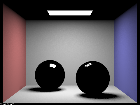
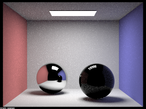
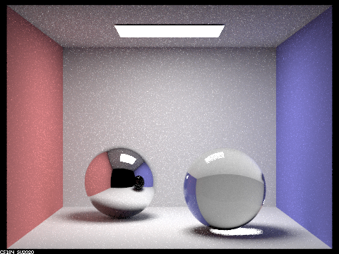
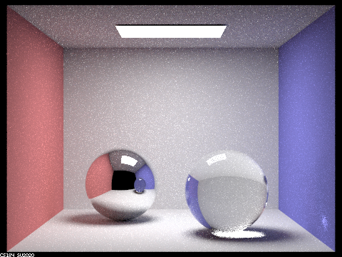
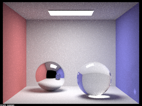
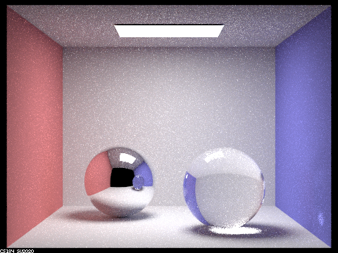
Parameters: -t 8 -s 64 -l 4 -m [variable] -r 480 360

|
|
|
|
|
|
|
We had a bug for a while where the refracted sphere was somewhat pixelated and had a black square plastered across its front side. We then realized that this was because we didn't set the pdf equal to 1 in our sample function!
Part 4: Depth of Field
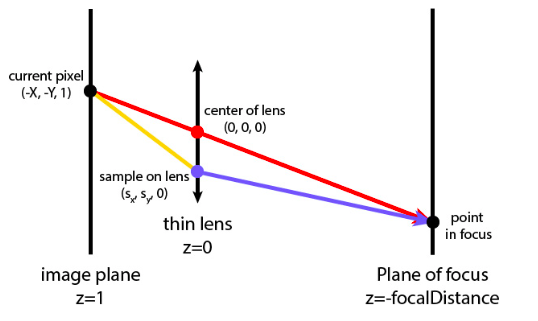
In previous projects, we used a pin-hole camera model. This is a model in which all the light intersecting a scene enters through a single point. This causes the effect of having everything in the scene be equally and fully in focus. However, real cameras have finite aperture sizes, so we implemented the thin-lens camera model to create more realistic renders. In this model, only objects in the plane focalDistance away from the lens are in focus. The focus worsens as you increase or decrease the depth from that plane. The thin-lens model also assumes that the thickness of the lens has negligible effect.
Previously, our ray tracer shot rays from the origin (0,0,0) toward some direction (X,Y,-1). Now, we uniformly sample the lens to get the sampled point on the lens at (S_x, S_y, 0) since we no longer recieve radiance from just (0,0,0). The formula to sample is:

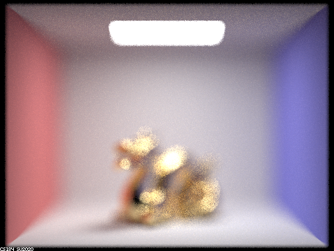
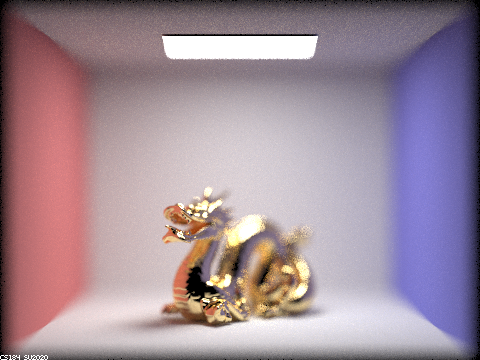
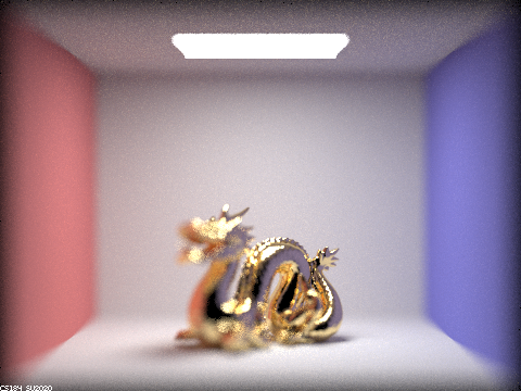
Below is a "focus stack" of a dragon image at 4 visibly different depths through a scene. The lens radius is set at 0.3. As the depth increases, we can see how the focused parts of the image shift from close to the lens to farther away. The first image has the bottom left corner in focus. The second and third images have the front and back of the dragon in focus. The last image has the back right corner in focus.
|
|
|

|
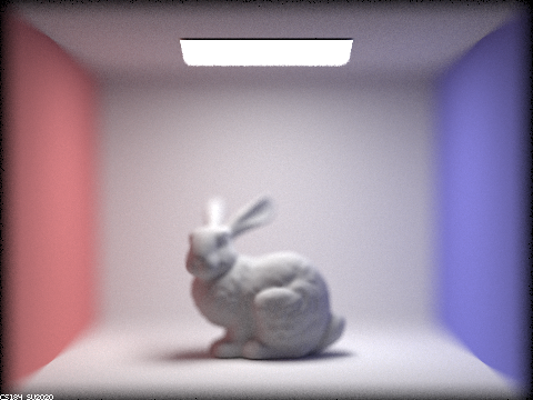
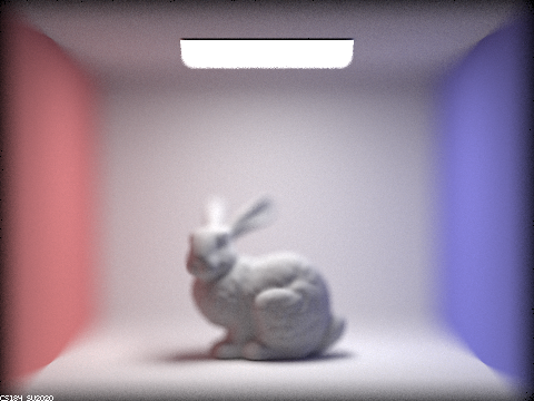
Below is a sequence of 4 bunny pictures with visibly different aperture sizes, all focused at the same point in a scene. The depth is set at 4.5. The first image is closest to the pin-hole camera model (lens radius = 0). As the aperture size increases, the difference in focus of objects at different depths increases. Take a look at the ears and face of the bunny to see this effect.

|

|
|
|
Our approach to this part of the project was to implement the steps directly from the spec and use the image of the rays in the spec to calculate our ray direction and origin. It was pretty straightforward from here. The only debugging issue we ran into was that we accidentally normalized both the origin and direction of the ray, instead of just the direction of the ray initially. What we learned from this part was exactly how aperture size affects focus and how important it is to be at a certain distance from the lens for an image to turn out well.
Partner work
We worked well as a team and as partners, each doing an equal amount of work. We both worked together on both parts of the project and debugged together in project parties and office hours. We also both contributed equally to the write-up. From past projects, we improved a lot with time management and worked over Spring break to finish early. Overall, it went greatly!