In this project, we implemented some fundamental algorithms of a physically-based renderer. These core components include ray generation and basic geometric intersections, constructing bounding voluming hierarchy trees, simulating light transport in different ways, and using Monte Carlo estimates for path tracing! Overall, we were able to render very realistic scenes with enough time and CPU power.
Part 1: Ray Generation and Intersection
1) Two parts of the rendering pipeline include ray generation and primitive intersections. Ray generation consists of taking normalized image coordinates, transforming them into camera space, generating the ray in camera space, and then transforming the ray into world space. Going from image coordinates to camera coordinates is essentially using the pixel plane on the image so that the ray can be drawn from the camera origin through the field of view. Going from camera space to world space with the correct direction displays the ray onto the scene. This ray generation technique is done for every pixel.
Once we are able to generate rays, we can test them for intersection with primitives in the scene. For triangle intersection, we used an algorithm called the Moller-Trumbore Algorithm, which does some vector math to compute the intersection value and uses barycentric coordinates for the intersection normals. As long as the intersection value was within the minimum and maximum values of the image and the barycentric coordinates were values between 0 and 1 and added up to 1, we had a valid value. We also implemented sphere intersection which involved using the quadratic formula. If we had no real roots, there was no intersection. If there was one real root, there was only one intersection and that was used to update the intersection data. For two real roots -- meaning two intersection points -- we use the closest intersection to update the intersection data.
2) As explained above, for triangle intersection we used the Moller-Trumbore algorithm. We can compute {{t, b1, b2}} = (1 / dot(s1, e1)) * {{dot(s2, e2), dot(s1, s), dot(s2, d)}} where e1 = p1 - p0, e2 = p2 - p0, s = o - p0, s1 = cross(d, e2), and s2 = cross(s, e1). t is the intersection value. o is the origin of the ray. d is the direction of the ray. p1, p2, and p3 are the planes of the triangle edges. b1 and b2 are barycentric coordinates, and we can find b3 by doing 1 - b1 - b2. As long as the intersection value was within the minimum and maximum values of the image and the barycentric coordinates were values between 0 and 1 and added up to 1, we had a valid intersection value. We update max_t of the ray to be the intersection value, t and the normal is computed using the barycentric coordinates as weights on the mesh normals.
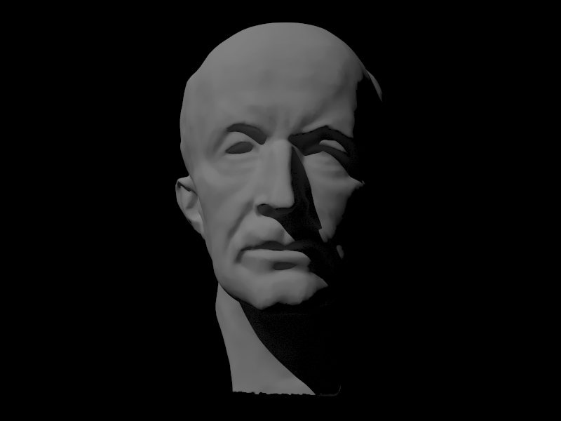
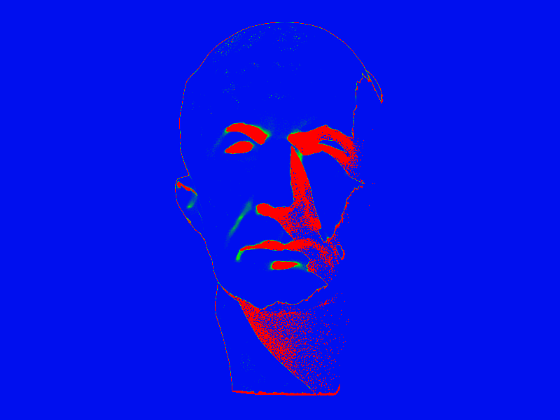
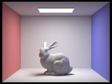
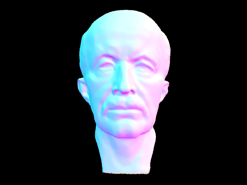
3) Here are some images with normal shading:
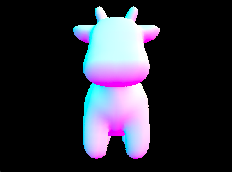
|
We didn't really have major debugging issues in part 1.
Part 2: Bounding Volume Hierarchy
1) When constructing the BVH, we first constructed the bounding box that contained the individual bounding boxes and areas of the given list of primitives included in the BVH. Then, we initialized a new BVHNode with this newly-constructed bounding box. If we find that we are at a leaf node (the number of primitives is less than the max leaf size), we updated the leaf nodes by setting the start and end. If not, we went through our recursive algorithm. The next step is to find our splitting point, using a heuristic. In order to determine our splitting point, we went along every axis (x, y, and z) and populated the primitives into left and right vector arrays for each axis based on where they lied with respect to the bounding boxs' average centroid locations. That is, we went along the x axis, split at the average centroid along the x axis, and populated vectors left_x with primitives with centroids to the left of the bounding box’s centroid, and populated vector right_x with primitives that have center values greater than or equal to average centroid location along the x-axis. We did the same thing along the y-axis and the z-axis. Then, we computed which axis had the most evenly split of primitives between the axes by finding the square of the difference in size between the left and right vectors for each axis. We squared this value to remove any negative signs that may have been introduced in the subtraction — we want to find the absolute difference! Finally, we populated the input vector with the values in our left and right vectors for the best axis split that we had (again, the most even one) and recused along the left and right sides of this split. To handle cases in which all centroids were at the same location or in general either one of the left or right vectors had been empty, we treated that node as a leaf node.
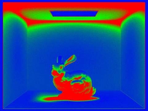
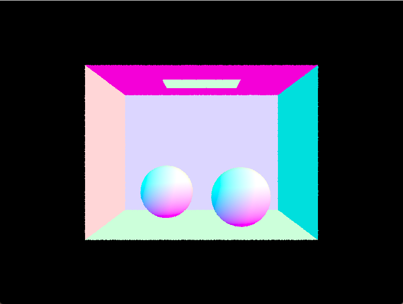
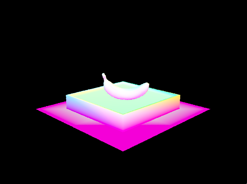
2) Here are some images rendered with BVH acceleration with normal shading:
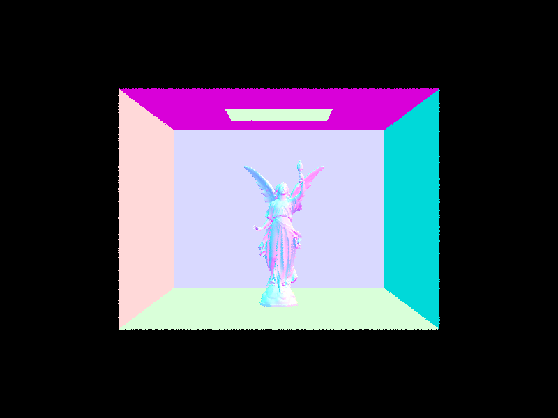
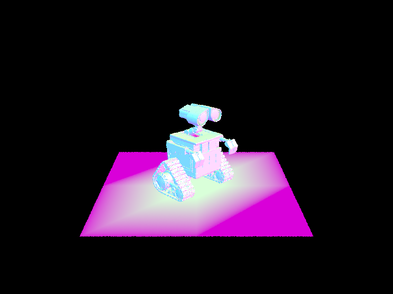
|
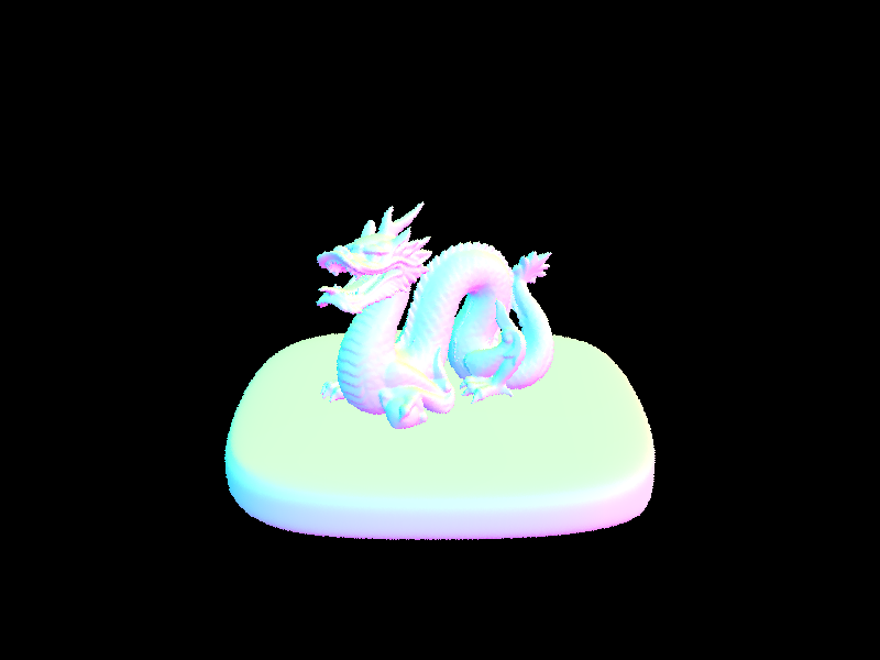
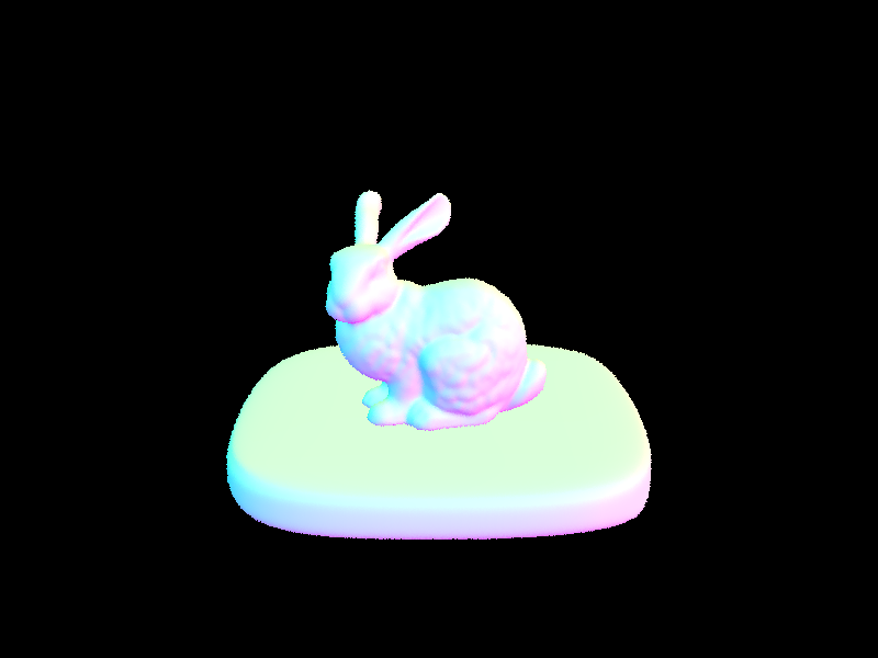
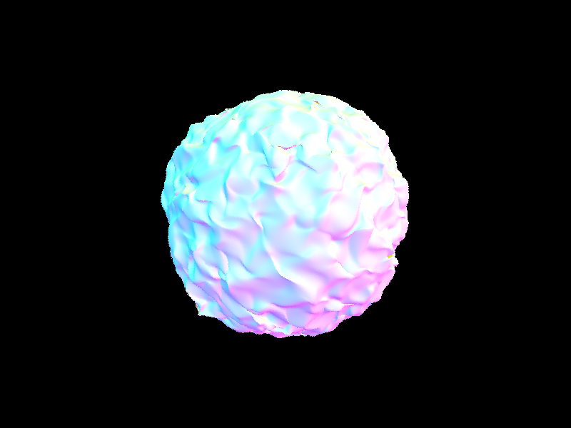
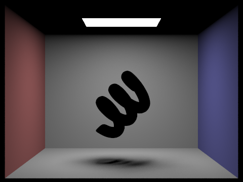
3) Below are a few scenes with moderately complex geometries with and without BVH acceleration. The dragon took 991.3042 seconds to render without BHV and 0.5524 seconds to render with BVH, an improvement of 990.7518 seconds.The bunny took 311.7275 seconds to render without BHV and 0.6602 seconds to render with BVH, an improvement of 331.0673 seconds. Finally, the blob took 2193.6462 to render without BVH and 2.4141 seconds to render with BVH. This improvement was 2191.2321 seconds! Rendering with BVH SIGNIFICANTLY reduced rendering time from minutes to within a second or a few. The blob showed the most dramatic difference, probably because the geometric surface was the most complicated of the three scenes.
|
The biggest debugging issue we had in part 2 was that we would segfault on some scenes and not others. After going to OH, we realized we did not handle the case in which either one of the left or right vectors was empty. To handle this, we treated that node as a leaf node and did not recurse. Another smaller issue we had at first is that our shading was not correct because we did not set the normal correctly in the sphere intersection function.
Part 3: Direct Illumination
1) Two different implementations were used for the direct lighting functions. In the first, we estimated the direct lighting on a point by sampling uniformly in a hemisphere. In our algorithm for hemisphere sampling, the number of times we sample is the number of lights in the scene times the area. The sample in object space is transformed into world space, and a ray using the sample is created that originates from our point of interest, hit_p. We need to integrate over all the light arriving in a hemisphere around the point of interest, so we use a monte carlo estimator to approximate it. We do the estimate for every ray going from the hit_p in the sampled direction that intersects a light source because we are only worried about direct illumination. For direct lighting, the estimator we used was (isect.bsdf->f(w_out, sample) * isect1.bsdf->get_emission() * sample.z) * (2 * PI). The reason we estimate how much light arrived at the intersection point from elsewhere is because we want to figure out how much light is reflect back toward the camera to determine the color of the ray thats cast from our camera through a specific pixel. Then, once we have an estimate of incoming light, we can use the reflection equation to calculate how much outgoing light there is. The relection equation is. We also used EPS_F as an offset for our ray.min_t.
In the second implementation, we used importance sampling which samples all lights directly, rather than uniform directions in a hemisphere. We do this because uniform hemisphere sampling can be noisy even though it can converge to the correct result. We can use this second implementation to render images that only have point lights. For all the samples in this algorithm, we sample the lights directly and get the distance to the light and pdf. For each light in the scene, we want to sample directions between the light source and the hit_p. We cast a ray in this direction and check that there is no other object between the hit point and the light source. If that's the case, we know that this light source does cast light onto the hit point, and we use the reflectance equation again to add onto our lighting estimate. The estimator we used for importance sampling was (isect.bsdf->f(w_out, wi) * radiance * dot(wi.unit(), isect.n.unit())) / pdf. We also used EPS_F as ray min and distToLight - EPS_F as ray max.
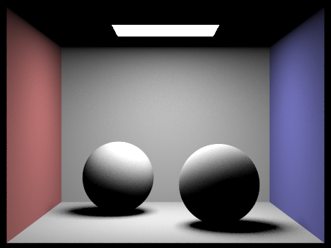
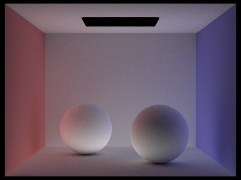
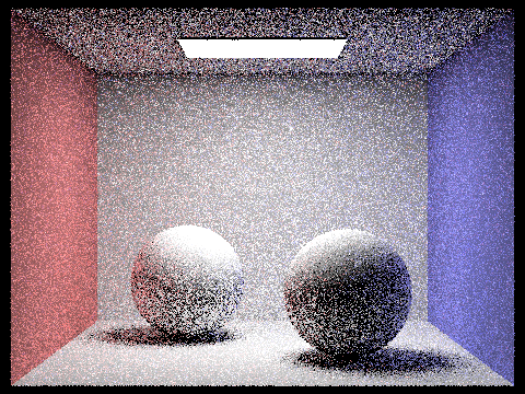
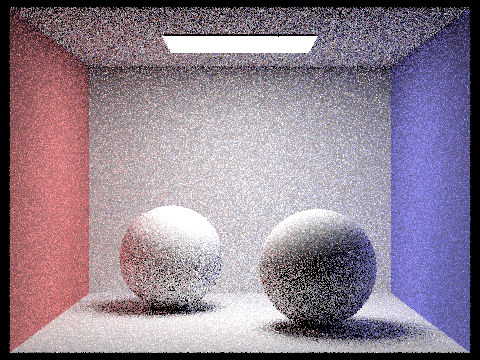
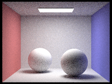
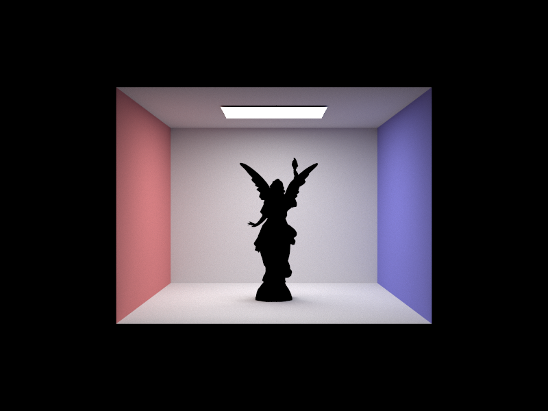
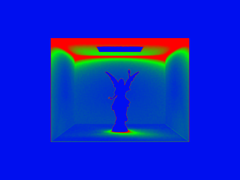
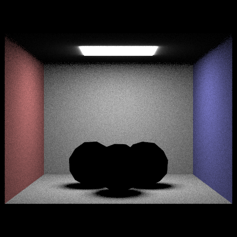
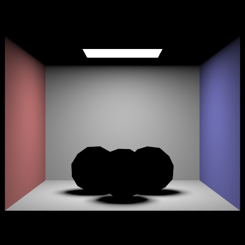
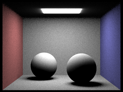
2) Show some images rendered with both implementations of the direct lighting function.
|
|
|
|
|

|
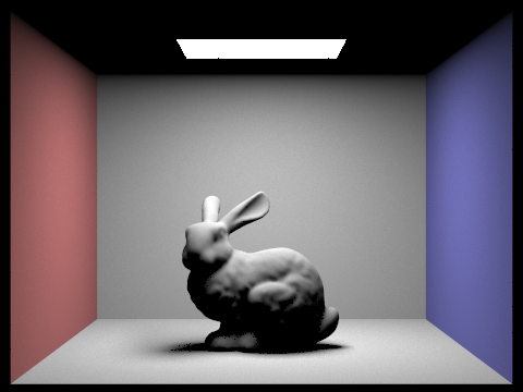
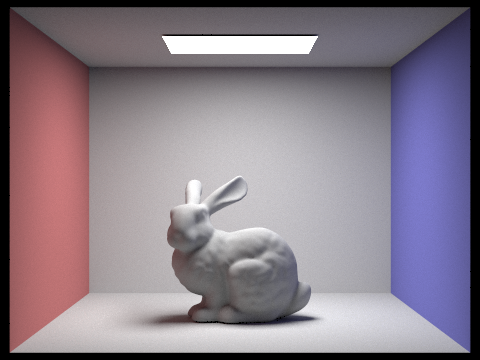
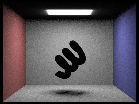
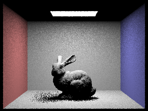
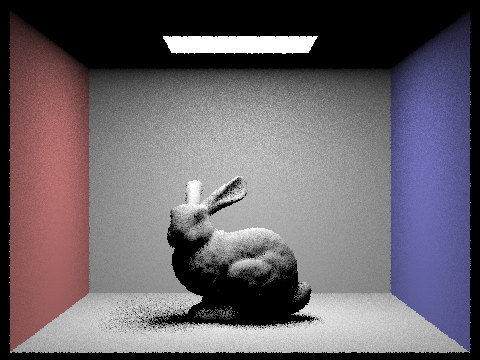
3) The following images of the bunny scene below are rendered with at least one area light, with 1 sample per pixel, using light sampling, and with a different number of light rays. If we take a closer look at the shadow underneath the bunny, we can see that the graininess of the soft shadow improves as the number of light rays increases. This shows us how light sampling is a good method to deal with noise in a scene, and how increasing the number of light rays also increases the image's clarity!
|
|

|

|
4) Uniform hemisphere sampling and lighting sampling are two methods to perform global illumination, but they have some key differences as you can see in the scenes of the coil, gems, and spheres above. The result of lighting sampling drastically reduces noise in images, best noticed when looking at areas with soft shadows. We see the resulting differences because of the way we sample the incident light ray directions in our estimation. In uniform hemisphere sampling, our ray samples do not necessarily point toward the light source. In importance sampling, they do because we specifically check if the ray intersects with another object in the scene and only add to the radiance if not. Using uniform hemisphere sampling converges to the correct result, but importance sampling does better using the same number of samples. The result is a smoother, less grainy image that keeps improving as we use more light rays.
One debugging issue we had with part 3 was that our shadows would be black, and some parts of the scene were too bright. What fixed it was setting cosine theta to the z vector was the sample (normal is 0,0,1) and messsing with other parameters like min_t and max_t to have the correct offsets.
Part 4: Direct Illumination
The indirect lighting function is essentially tracing the incoming ray from the light to a certain depth / number of bounces. When we’re calling this function, we know we will always be doing at least one bounce. As such, the first thing we do in the function is set our final illumination effect on the scene to be a vector that results from one bounce of the ray. Then, we begin our algorithm. For the first ray incoming in the scene — that is, the ray that directly comes from the light source — we should always recurse at least one time, meaning it does two bounces. However, this should only take place if the maximum depth is greater than 1, because that means it should bounce more than 1 time! In this case, since we want all light rays to bounce / recurse at least once if their depths allow for that, we do not take russian roulette into account. That is, because russian roulette then gives the possibility of terminating the recursion before it begins. We implement this in the check if the (max_ray_depth == r.depth) && r.depth > 1, which essentially is checking that this is the first time this function has been called on the input ray (since the ray is initialized to max_ray_depth and its depth decrements at every recursive call), and checks that the depth is valid to recurse. Once inside the if statement, we create a new ray that represents this incoming ray in the world space. In order to create this ray, we take a random sample of an incoming ray direction. We set the minimum t value of the ray to be EPS_F to account for slight errors, and decrementing ray's the depth by 1 (setting it equal to r.depth - 1) because it is the next ray in the traversal sequence and therefore has one less "depth" than r. Then we check if the world ray intersects with a location in the scene. If it does, we know that the ray will interact with the scene on future bounces, and therefore we must continue following the ray’s bounce. So, we recurse! One thing to note here is that our calculation of the illumination is different depending on what ray we are looking at. If we are recursing after the very first bounce, that means that russian roulette did not play a part in it being shown in the scene, and we therefore should not divide by the cpdf (1 - termination probability due to russian roulette). We know it's on the first bounce, again, because the depth of the current ray has not been decremented yet. However, at all other ray cases / depths, we do divide by the cpdf because in order to enter the if statement, it passed through the russian roulette random termination!