Overview

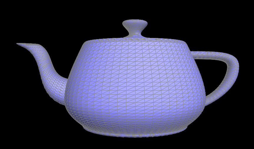
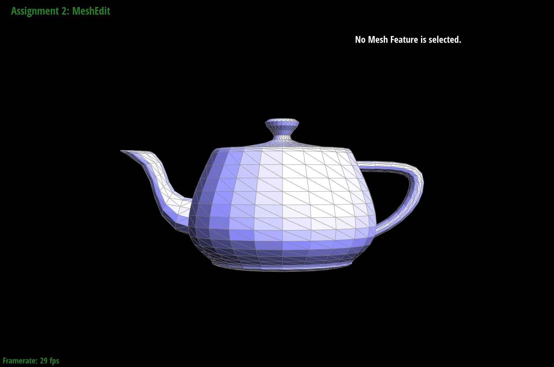
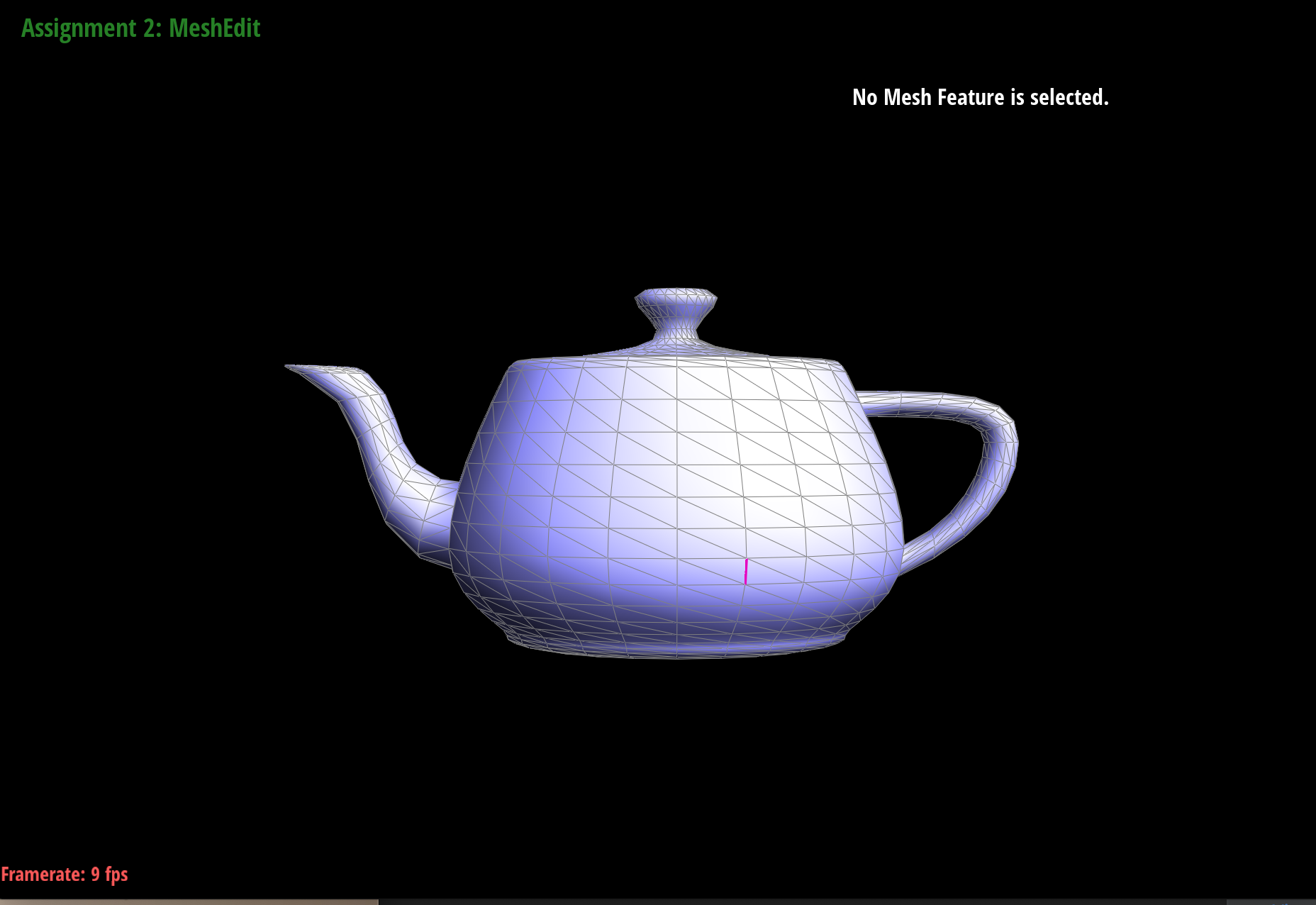
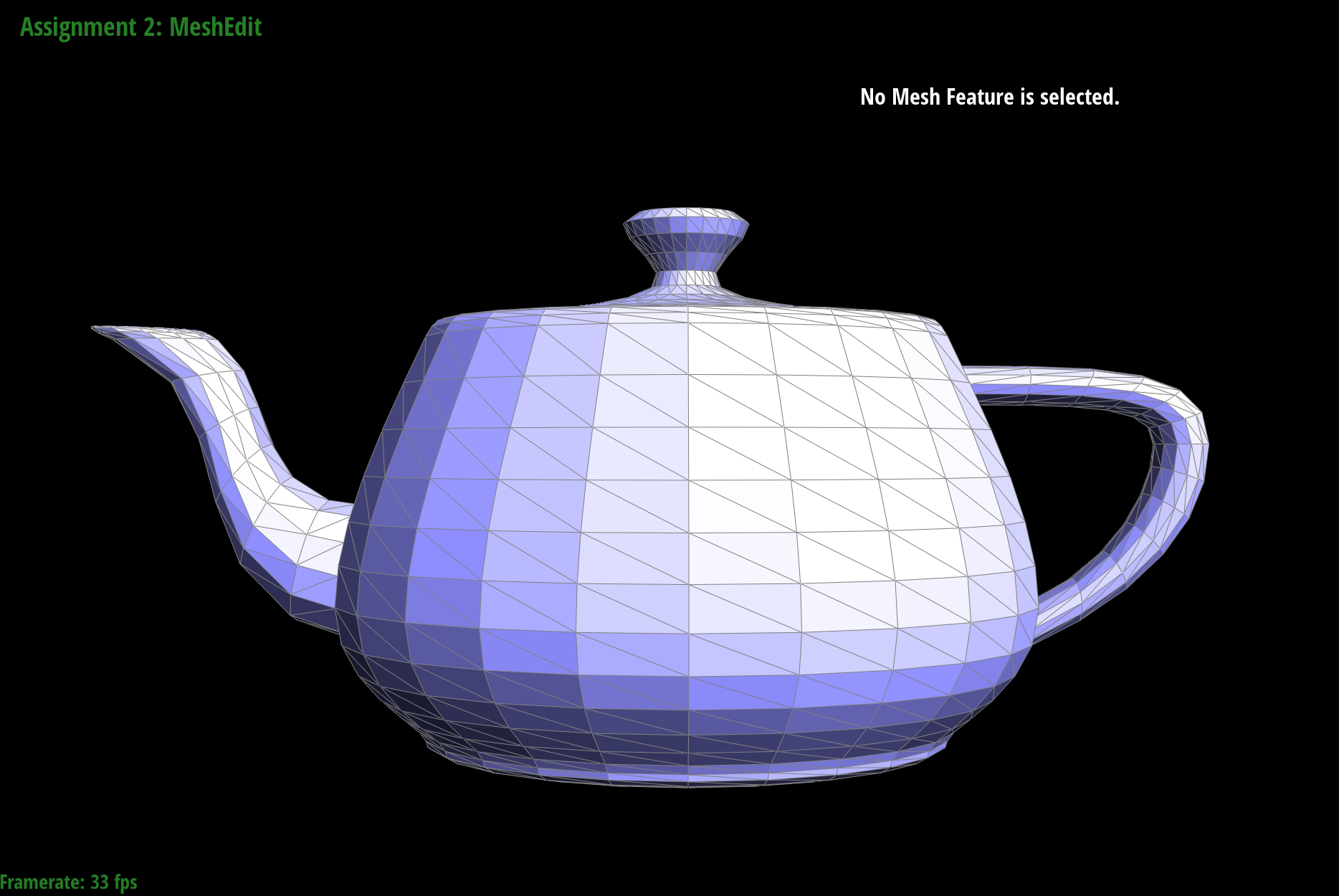
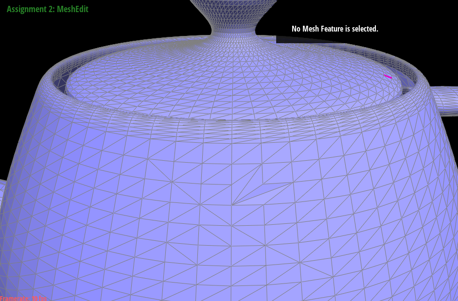
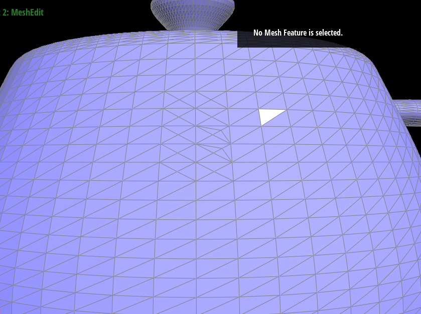
In this assignment, we implemented important techniques for geometric modeling. We built Bezier curves and surfaces using de Casteljau algorithm, manipulated triangle meshes represented by half-edge data structure, and implemented loop subdivision. An interesting thing we learned was how big of a difference in texture and shading it makes when we alternate between flat shading and more advanced methods like phong shading. With the particular example of the teapot, this difference was much more dramatic than we initially expected.

Section I: Bezier Curves and Surfaces

Part 1: Bezier curves with 1D de Casteljau subdivision

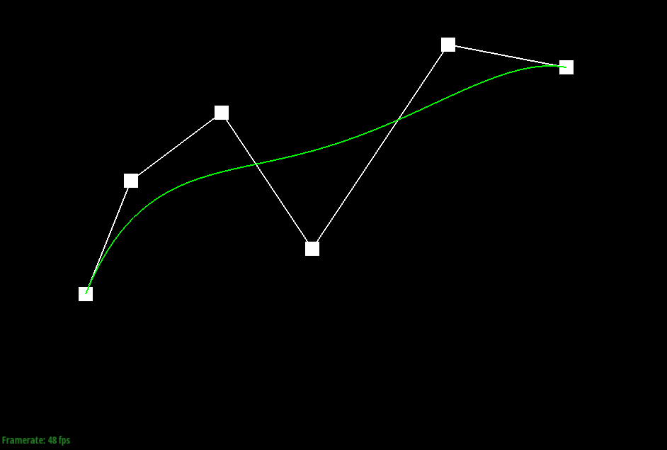
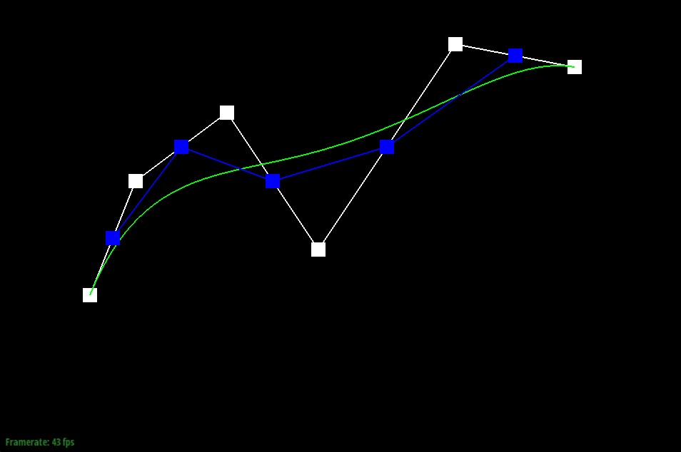
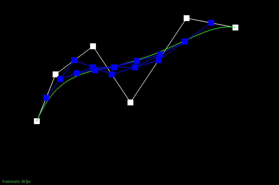
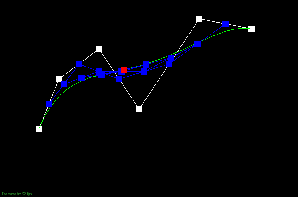
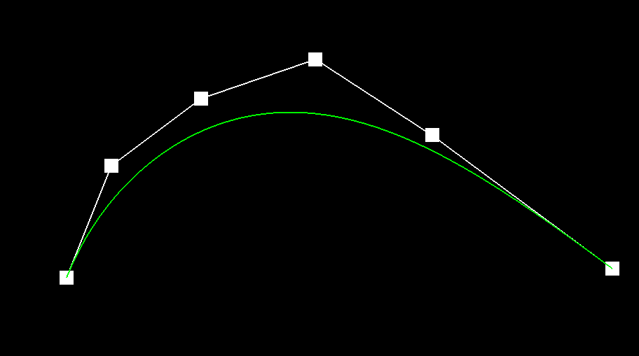
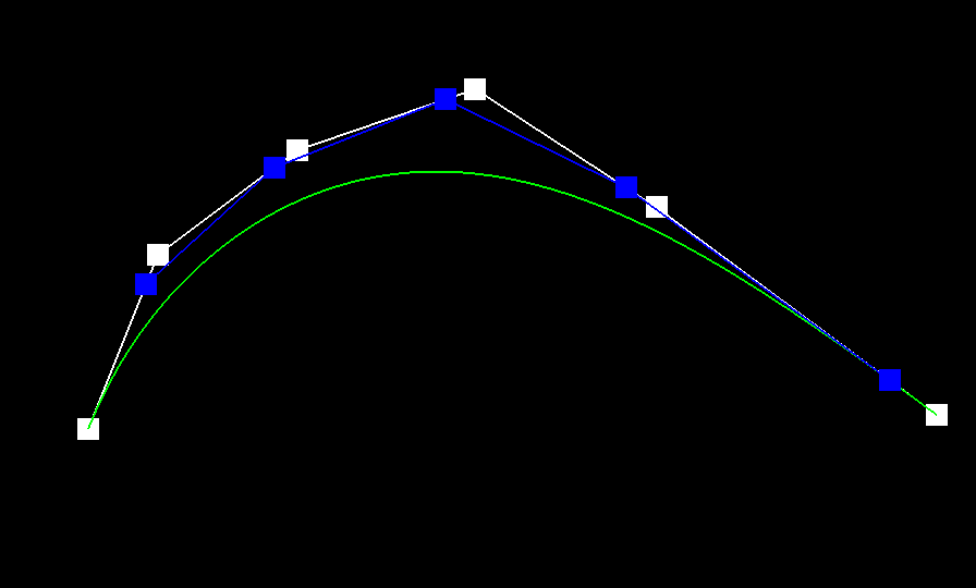
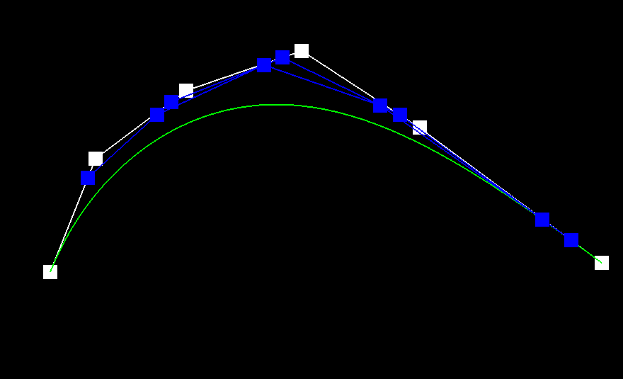
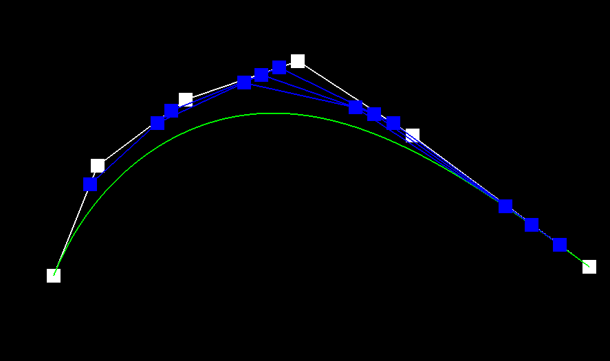
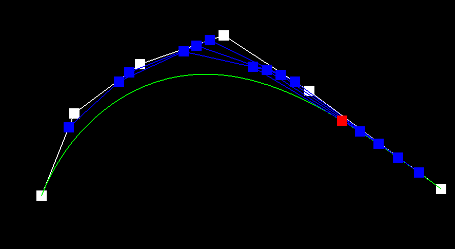
1) de Casteljau’s algorithm is a way to evaluate polynomials for n-degree curves by continually linearly interpolating adjacent points. In the case of this project, we are given n control points, which gives us our approximate curve. By linearly interpolating adjacent points — in this case, p0 and p1, p1 and p2, and so on — with a weight t, we are able to continue recursively running the algorithm on our n points, subdividing them until they are reduced to one single point. This calculation is modeled by pi′ =lerp(pi,pi+1,t)=(1−t)pi+tpi+1). This final point, combined with the given starting and ending point, results in the final Bezier curve.

2)

3)

Part 2: Bezier surfaces with separable 1D de Casteljau subdivision

1) de Casteljau algorithm extends to Bezier surfaces by doing the same operation and steps as detailed in part 1’s 1D Bezier curve implementation, but in 3 dimensions (so for 3D vectors rather than the 2D vectors). In order to do this, we calculate all of the 1D interpolations in one direction by running de Casteljau algorithm on them, and then take those new points and run de Casteljau algorithm on them, which in effect will run it in the other dimension. So, in the implementation, we iterate through the given controlPoints, which is a 2D array of vector points. Every index of the control points is a set of vertices we can run the algorithm on, and the algorithm returns one vector that we added to an array of vectors (int_vect). Then, we were able to evaluate that array of vectors by interpolating one last time, and that will return the final interpolated vector for the Bezier surface!

Section II: Sampling

Part 3: Average normals for half-edge meshes

1) In order to implement the area-weighted vertex normals, the first step was to iterate through every face incident to the given vertex. As such, our while loop’s condition is when h != halfedge() because we will only cease iterating once we’ve reached the edge from which we started, which ensures that we don’t add repeat face values to the sum. We also only include the face if it is not a boundary. As we iterate through the faces, we keep track of the weighted sum of the faces (represented by face_normal * face_area) in the variable area_weighted_normals_sum. The weighted sum of the face is represented by (face_normal * face_area) because the normal vector of the face needs to be weighed appropriately based on how much space it takes up in the mesh / how much effect it would have on the face’s normal. Once we’ve calculated the sum, resulting in a vector pointing in a direction, the correct direction, as computed by the weighted faces. Finally, on our area_weighted_normals_sum, we normalize the sum using the given unit() method.

2)

Part 4: Half-edge flip

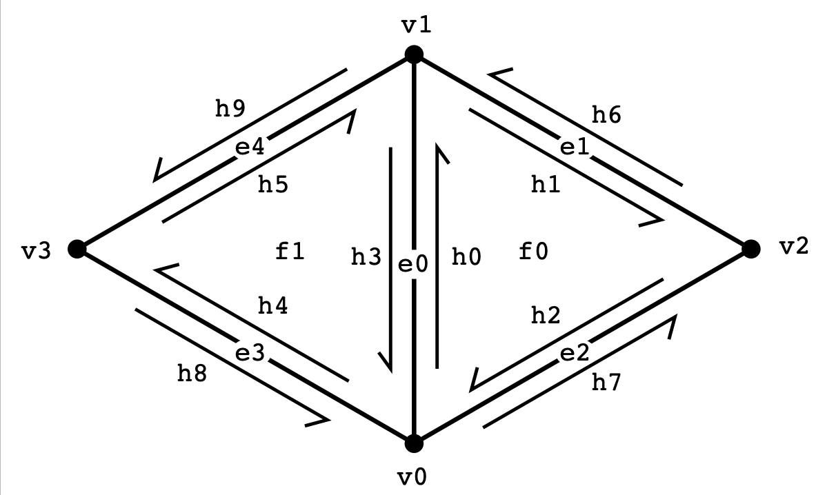
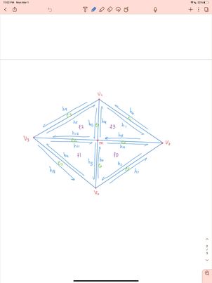
1) In order to avoid very intensive debugging, we spent a long time creating and validating our “before” and “after” diagram [ATTACHED]. After creating his diagram, we found CMU’s “Guide to Implementing Edge Operations on a Halfedge Data Structure” that was linked on Piazza, which actually was incredibly similar to the diagram we had created. Since the guide’s diagram was much easier to understand and parse, we decided to use this implementation pattern in our code. We decided that the most straightforward way to implement this transformation would be to first define all of the existing faces, vertices, half edges, and edges in the “before” diagrams, defining each struct by its position with respect to the given edge iterator e0. After defining this, we performed the flip operation. This entailed simply looking at out “after” diagram and reassigning the half edge, edge, vertex, and face relationships and values to correspond to what we had already mapped out in the diagram. This worked because we had already set up the “before” state, so we were accurately transforming the given edges based on the schema we had devised and established earlier. Our debugging just entailed looking closely through our assignment statements and ensuring that we had assigned it properly according to our diagram, fixing any typos we may have made.

2)

3) We didn't really experience an eventful debugging journey considering we mostly referenced the code in the guide provided to us.

Part 5: Half-edge split

1) The implementation for split edge, in practice, ended up being quite similar to the implementation for flip edge — assign your starting half edges, edges, faces, and vertices, perform an operation, and then reassign the values to their final position. Our structs, to begin with, were defined exactly the same way as in flip edge, for consistency. At the end of the day, it likely didn’t make a difference, but it definitely helped us wrap our minds around the context of the problem! After defining our starting state, we created 1 new vertex, 3 new edges, 6 new half edges, and 2 new faces. The new vertex m is the midpoint of the given edge, which is where the split is actually taking place. That midpoint connects to points a and d (as shown in the diagram in the spec), for which we must create 2 new edges and 4 half edges (the edges and their respective twins). Because we’re splitting edge bc in half, that edge and its half edges can be refactored into the edge bm.

2)

3)

4) Our debugging journey was pretty simple. We just went through the diagram we made more more time and realized we misassigned one pointer.

Part 6: Loop subdivision for mesh upsampling

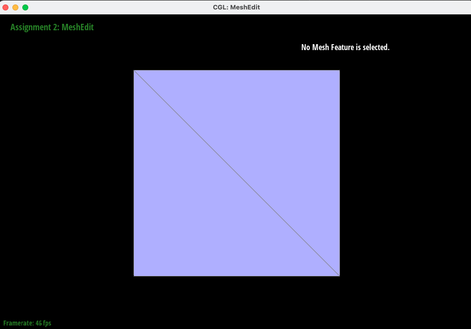
For loop subdivision, we used the implementation recommended in the spec that includes 4-1 subdivision and splitting and flipping edges. First, we computed new positions for all original vertices in the mesh. In order to do so, we created a helper function, NewPosition. In this helper, we essentially calculated the sum of all neighboring vertices using half edge and twin traversals, continually adding neighboring vertices until we circled back and retraversed over the same half edge that we began with. Then, we used the equation detailed by the diagram in the spec using (1 - n * u) * original_position + u * original_neighbor_position_sum where n is the degree of the vertex and u is 3/16 if n=3 and 3/8n otherwise. Then, we iterated through all edges present in the original mesh to calculate the values of what the "midpoint" vertices would be if and when that particular edge would be split. In order to do this, we looked through the two vertices on either side of the edge along with the two vertices perpendicular to them, labelling these vertices a, b, c, and d in accordance with the diagram in the spec. For each edge, we compute the new vertex using the equation 3.0/8.0 * (a->position + b->position) + 1.0/8.0 * (c->position + d->position) and set that in its newPosition attribute. One issue we had here was actually with the float values -- we used 3/8 and 1/8 rather than 3.0/8.0 and 1.0/8.0 which gave us an incorrect answer! Then we split all edges in the mesh and flip the ones connecting old and new vertices. Voila, that’s loop subdivision! The newPosition and splitEdge methods ended up being a large part of our debugging journey. At first, we set all vertices and to be not new (isNew = 0) in those methods, but after some time realized that was faulty and decided to add the aforementioned for loop at the beginning, which was used to explicitly make every original vertex labelled as such. In this method, we also added a check to see if the edge being split was new -- if it was, we found the midpoint by averaging the two edge vertices, and if it wasn't, we used the value we specified in the edge's newPosition attribute. Before fixing these two things, our mesh was very inwardly-pointing and did not smooth properly. A final issue we had with this was setting our vertices all to their newPosition, rather than just the old ones. When we set all vertices as such, it resulted in a black screen because many of our points were overwritten and set to a position (0,0,0), which was not our intended effect.

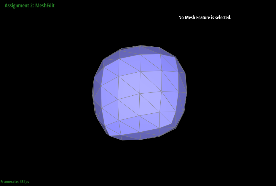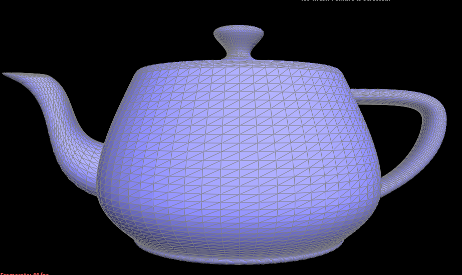
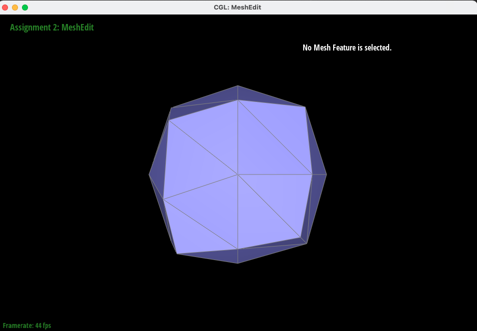
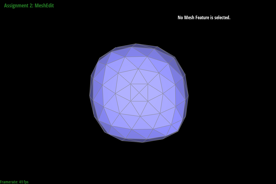
As the figure is subdivided further and more edges and vertices are added, its sharp corners and edges get smoothed out!

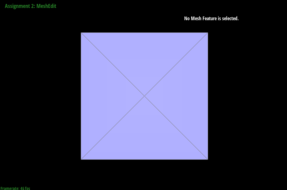
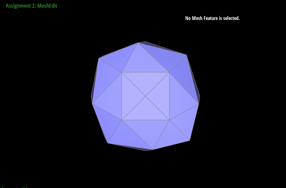
Because we added the split at the beginning, it divided more symmetrically. Since the cube begins with one diagonal edge across the front, it ends up subdividing around that line (because loop subdivision is dependent on the edges in the mesh), which ultimately led to a somewhat skewed shape. By evening out the number and location of the edges on the forward facing part of the mesh (in this case, making it an "x" shape ), it made our loop subdivision even as well. When I tried to split edges after subdividing once or twice, it was much more difficult to alleviate. That's because you not only have to evenly split and anticipate which split edges would even out the mesh in further subdivisions, but there are also many more boundary edges that are not allowed to be split and can lead to some interesting but not necessarily symmetric shapes. By pre-processing at the very beginning, it reduces these extra complications that one may run into further down the line when there are more edges and effects to consider (every edge split has a smaller effect on the mesh the more you subdivide, so it makes most sense to make the edges symmetrical at the very beginning)!